Excel and Tableau : Basic - Moderate Concepts.

Excel and tableau are the best analytical tools being used in the various fields. And It is very essential for the ones who are enhancing there career towards Data Analytics. In this article I would like to provide detail overview about the basic formulas and concepts that are being used in excel and tableau.

Excel

1. Operator Precedence : If a part of the formula is in parentheses, that part will be calculated first. It then performs division, multiplication, Addition or subtraction (BODMAS) calculations.

Ex: 1+3*2+(6/2)-10 = 0

Illustration : > Parentheses will executed first : =1+3*2+3-10.

> Multiplication second : =1+6+3-10

> Addition Third : =10-10

> Subtraction : =10-10

Answer = 0. 2. COUNT vs COUNTA : COUNT - Counts the numbers of cells in a range which contains only numeric.

COUNTA - Counts the number of cells in a range that are not empty. ex: COUNT

Ex: COUNTA

3. COUNTIF : Counts the number of cells within a range that meets the given criteria.

4. SUMIF : Adds the cells specified by a given condition or criteria.

5. IF Function : The IF function checks whether a condition is met, and returns one value if true and another value if false.

Expression : IF(logical_test, value_if_true, value_if_false)

Ex:

6. If with AND, OR functions :

A. If with And function : Expression : And(logical2,logical2,...)

The AND function returns TRUE if the first value is greater than or equal to 60 and the second score is greater than or equal to 90, else it returns FALSE. If TRUE, the IF function returns Pass, if FALSE, the IF function returns Fail.

B. If with OR function : Expression : Or(ogical1,logical2,....)

The OR function returns TRUE if at least one score is greater than or equal to 60, else it returns FALSE. If TRUE, the IF function returns Pass, if FALSE, the IF function returns Fail.

C. If with And - OR function :

The AND function below has two arguments separated by a comma (Furniture, Green or Blue). The AND function returns TRUE if Product equals "Furniture" and Color equals "Green" or "Blue". If TRUE, the IF function reduces the price by 50%, if FALSE, the IF function reduces the price by 10%.

=IF(AND(A8="Furniture",OR(B8="Green",B8="Blue")),0.5*C8,0.9*C8)

Formula Interpretation :

> If Product = Furniture and color = (Green or Blue) then 50 % off C8 (Price).

> If Product <> Furniture then the condition right away calculate the 90% off C8 (price), Here the first condition itself failed hence it will not further reference or condition.

7. Nested-IF : One IF function inside another, allows you to test multiple criteria and increases the number of possible outcomes.

If the score equals 1, the nested IF formula returns Bad, if the score equals 2, the nested IF formula returns Good, if the score equals 3, the nested IF formula returns Excellent, else it returns Not Valid.

8. VLOOK-UP

Vlookup Looks Right

The VLOOKUP function always looks up a value in the leftmost column of a table and returns the corresponding value from a column to the right.

In its simplest form, the VLOOKUP function says:

=VLOOKUP(What you want to look up, where you want to look for it, the column number in the range containing the value to return, return an Approximate or Exact match – indicated as 1/TRUE, or 0/FALSE).

The VLOOKUP function below looks up the value 6 (first argument) in the leftmost column of the green table (second argument). The value 4 (third argument) tells the VLOOKUP function to return the value in the same row from the fourth column of the green table.

=VLOOKUP(F2,A2:D8,4,FALSE) : Illustration.

F2 (lookup_value) = Lookup value i.e - 6.

A2:D8 (table_array) = Array in which we are looking for the value.

4 = The vlookup function to return the value in the same row from the 4th column of the green table.

9. VLOOK - UP Approximate Match :

The Boolean TRUE (fourth argument) tells the VLOOKUP function to return an approximate match. If the VLOOKUP function cannot find the value 85 in the first column, it will return the largest value smaller than 85. In this example, this will be the value 80.

10. Vlookup is Case-insensitive:

The VLOOKUP function in Excel performs a case-insensitive lookup. Explanation: the VLOOKUP function is case-insensitive so it looks up MIA or Mia or mia or miA, etc. As a result, the VLOOKUP function returns the salary of Mia Clark (first instance).

11. Index with Match Function : INDEX - returns the value of a cell in a table based on the column and row number.

MATCH - Returns the position of a cell in a row or column.

INDEX and MATCH is incredibly flexible – you can do horizontal and vertical lookups, 2-way lookups, left lookups, case-sensitive lookups, and even lookups based on multiple criteria.

A. Match Function :

The MATCH function returns the position of a value in a given range. For example, the MATCH function below looks up the value 6161 in the range X4:X9.

B. Index Function :

The INDEX function returns the 5th value (second argument) in the range AA4:AA10 (first argument).

Expression : INDEX(AA4:AA10,5) = 58339.

C. Index & Match Results :

=INDEX(AA2:AA8,MATCH(AD3,X2:X8,0))

Illustration : =INDEX(AA2:AA8,MATCH(AD3,X2:X8,0))

AA2:AA8 = array,

AD3 = lookup_value,

X2:X8 = lookingup_array

0 = Exact match.

12. Index & Match - Two Way Look-up:

The INDEX function can also return a specific value in a two-dimensional range. For example, use the INDEX and the MATCH function in Excel to perform a two-way-lookup.

13. Case-sensitive Lookup

By default, the VLOOKUP function performs a case-insensitive lookup. However, you can use the INDEX, MATCH and the EXACT function in Excel to perform a case-sensitive lookup. {=INDEX(AS22:AS28,MATCH(TRUE,EXACT(AV22,AQ22:AQ28),0))}

10. Average Function : The Excel AVERAGE function calculates the average of supplied numbers. =AVERAGE(C75:C78-B75:B78)

1. 14. Index and match with multiple criteria

Generic formula : We need to use f9 in window to execute this formula.

{=INDEX(range1,MATCH(1,(A1=range2)*(B1=range3)*(C1=range4),0))}

This formula works around this limitation by using Boolean logic 1 and 0 to create an array of ones and zeros to represent rows and matching all 3 criteria, then using match to match the first 1 found. The temporary array of ones and zeros is generated with this snippet.

Example : In the world of Boolean algebra, there are only two possible values for a math operation: 1 or 0. Boolean logic refers to a technique of building formulas to take advantage of the fact that TRUE = 1, and FALSE = 0. In Excel, any math operation will coerce TRUE and FALSE values into 1's and 0's. In the example shown:

=(C5>=90)*(D5="Super")=(TRUE)*(TRUE)=1

Formula Used : {=INDEX(D10:D17,MATCH(1,(H10=A10:A17)*(H11=B10:B17)*(H12=C10:C17))}

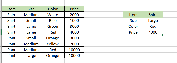
(H5=B5:B11)*(H6=C5:C11)*(H7=D5:D11)

Here we compare the item in H5 against all items, the size in H6 against all sizes, and the color in H7 against all colors. The initial result is three arrays of TRUE/FALSE results like this:

{TRUE;TRUE;TRUE;FALSE;FALSE;FALSE;TRUE}*{FALSE;FALSE;TRUE;FALSE;FALSE;TRUE;FALSE}*{TRUE;FALSE;TRUE;FALSE;FALSE;FALSE;TRUE}

The math operation (multiplication) transforms the TRUE FALSE values to 1s and 0s:

{1;1;1;0;0;0;1}*{0;0;1;0;0;1;0}*{1;0;1;0;0;0;1}

After multiplication, we have a single array like this:

{0;0;1;0;0;0;0}

which is fed into the MATCH function as the lookup array, with a lookup value of 1:

MATCH(1,{0;0;1;0;0;0;0})

At this point, the formula is a standard INDEX MATCH formula. The MATCH function returns 3 to INDEX:

=INDEX(E5:E11,3)

and INDEX returns a final result of 4000.

Tableau

Tableau : connecting, analyzing, and sharing. connecting to data, analyzing it using essential charts, and creating an interactive dashboard for sharing your views.

1. Some Important Definitions and Notes :

1. Data granularity refers to the level of detail for a piece of data, wherever you are looking. As data becomes less granular, we might describe it as an aggregation, or as aggregated data.

2. Aggregation refers to how data is combined. The level of granularity or aggregation in a row or chart affects the questions we can ask of the data, and the discoveries we can make.

3. A field, also known as a column, is a single piece of information from a record in a data set.

4. Qualitative Dimensions :

A. Describes or categorizes data

B. Tells you what, when, or who

C. Slices the quantitative data

5. Quantitative Measures :

• Numerical data

• Provides the measurement for qualitative category

• Can be used in calculations

2. Data Types:

1. Text or string values.

2. Discrete date and time field.

3. Discrete date field.

4. Geographic field (State, Zipcode).

5. Continuous Numeric Value.

6. Calculated filed.

3. Quick Table Calculation Overview:

A. Difference From.

ex : Current month 81921 - last month 201021 = -119100

B. Running Total.

C. Percent of total :

Current month sales 202021/grand total 923592 * 100.

D. Percent from :

ex : Feb month sales 470533/ Jan mon sales 484247 * 100

4. Calculations work with aggregation.

If we are not paying attention to how tableau automatically aggregates data, we may not get the results we want. A common example of this is ratio calculation. Here, We have profit / sales. In the view tableau automatically aggregates it, resulting in a field that looks like this.

Tableau calculates the ratio for each row then it would sum the results of these ratios. Sum the results is not very helpful what we really want here is to change the order of operations.

Ex: Sum(Profit/Sales) = 5340.17% Sum(Profit)/Sum(sales) = 618.99%

5. KPI - Key Performance Indicator:

A key-performance indicator is a metric that demonstrates how effectively you are achieving a key business objective.

Sample data :

Step 1 : Drag the dimension to rows (month) and KPI target and actual sales to column.

Step 2 : Change the KPI target to dual axis.

Step 3 : In the marks section change the KPI target to bar chart, color pallet to green and actual sales into the bar as well.

Step 4 : Go to the actual sales and reduce the bar size.

Step 5 : Synchronize the axis.

Step 6 : On the KPI target axis right click and add reference line. And make the following changes. Sum(Profit target) = total, per cell. Lable = None.

6. Percent difference from fixed to a particular dimension along with filtering the top 10 values.

Many of you might have faced difficulties in filter the top values for a dimension based on the percent difference from. In this article will provide the solution for this.

> The following formula will get you the percent difference from, from the previous year.

{ FIXED [State] : SUM(IF DATETRUNC('year',[Order Date])={FIXED : MAX(DATETRUNC('year',[Order Date]))} THEN

CASE [Parameters].[Measures]

WHEN 'Sales' THEN ([Sales])

WHEN 'Profit' THEN ([Profit])

END END)}

/{ FIXED [State] : SUM(IF DATETRUNC('year',[Order Date])=DATEADD('year',-1,{FIXED : MAX(DATETRUNC('year',[Order Date]))}) THEN

CASE [Parameters].[Measures]

WHEN 'Sales' THEN ([Sales])

WHEN 'Profit' THEN ([Profit])

END END) }

-1

Interpretation of the above formula. 1. Fixed : Computes an aggregate using only the specified dimensions. (At data source level). 2. DATETRUNC : Truncates the specified date to the accuracy specified by the the date part and returns the new date.

ex: datetrunc('month',#2001-09-10#) = 2001-09-01

3. MAX(DATETRUNC('year',[Order Date])) : Returns the max

In the next phase, I will add more information about : Dual - Axis, Fixed, Include, exclude, Working strings, dates and type conversion functions, Statistics and forecasting and Advanced functions and data analysis.