
SQL Analytical Functions
- Gowtham V

- Jun 4, 2022
- 7 min read
Updated: Sep 18, 2022
Analytical functions are one of the most popular tools among BI/Data Analysts for performing complex data analysis. These functions perform computations over multiple rows and return the multiple rows as well. Today we'll cover some important and most useful Analytical functions.
Points To Be Remembered :
* Analytical functions are functions that calculate an aggregated values based on group of rows.
* Aggregate functions calculate aggregated value for a result set, which must be grouped by the columns in select statement or to find an overall value. But with analytical functions, however, you can group the data that is used to calculate the functions result but show a value one each record in the result set, without grouping.
An analytical function generally looks like this.
Syntax
analytic_function_name([argument_list]) OVER ([PARTITION BY partition_expression,…]
[ORDER BY sort_expression, … [ASC|DESC]])
Many of the aggregate functions can also be used as analytical functions
Ex:
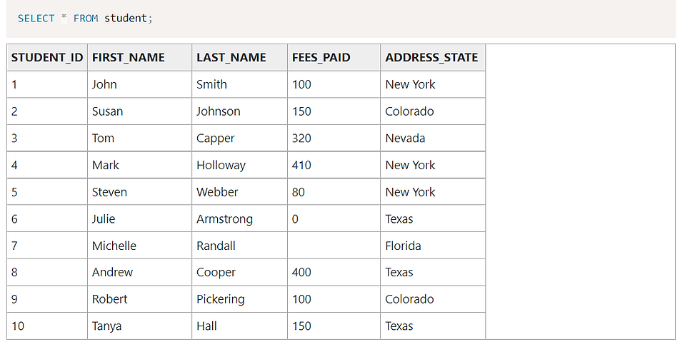
* What if you want to find the number of students in each state, and display that next to student record?

This would work, but it would only show the states and the count. It doesn’t show the student information.
I could add the student information, but then the COUNT(*) records would only show 1 because they are grouped by the student’s first_name and last_name.
This is where analytic functions come in.
The COUNT function as an analytic function would look like this:
COUNT(*) OVER (PARTITION BY address_state)This will find the COUNT of records for each state – but will not require any grouping in the SELECT statement.
SELECT first_name,
last_name,
address_state,COUNT(*) OVER (PARTITION BY address_state) AS state_count
FROM student;
Select first_name, last_name, address_state, count(*) over (partition by address_state) as state_count from student;

* What is partition by clause?
As you can see in the earlier example, the PARTITION BY specifies how the function groups the data before calculating the result.
* It works similar to a GROUP BY, but it doesn’t reduce the number of rows that are shown in the result set.
* If you don’t include the PARTITION BY, then you’ll get this result:
Select first_name, last_name, address_state, count(*) over() as state_count from
student;

When Are Analytic Functions Performed?
When the database processes a query, the analytic functions are the last set of operations performed, except for the ORDER BY clause. This means that the joins, the WHERE clause, GROUP BY clause, and HAVING clause are all performed first, then the analytic functions are performed.
This also means that the analytic functions can only appear in the SELECT list or the ORDER BY clause.
analytic_function_name: name of the function — like RANK(), SUM(), FIRST(), etc
partition_expression: column/expression on the basis of which the partition or window frames have to be created
sort_expression: column/expression on the basis of which the rows in the partition will be sorted
-----------------------------------------------------------------------------------------------------------------------------------------
Important Notes:
Window Functions
* Different categories of window functions.
Aggregate functions : Avg, Sum, Count,Min, Max
Ranking Functions : Rank, Dense_rank,Row_Number etc.
Analytical functions : Lead, Lag, First_value, Last_value etc.
Over clause defines the partitioning and ordering of the rows(i.e window) for the above functions to operate on. Hence these functions are called window functions. The over clause accepts the following three arguments to define a window for these functions to operate on.
* Order by : Defines the logical order of rows
* Partition by : Divides the query result set into partitions. The window function is applied to each partition separately.
* Rows or Range Clause : Further limits the rows within the partition by specifying start and end points within the partitions.
The default for rows or range clause is
* Range between unbounded preceding and current row.
UNBOUNDED PRECEDING indicates that the window starts at the first row of the partition; offset PRECEDING indicates that the window starts a number of rows equivalent to the value of offset before the current row. UNBOUNDED PRECEDING is the default. CURRENT ROW indicates the window begins or ends at the current row.
.

I.E Starts with in the beginning and ends with the last row.
* ROWS BETWEEN 1 PRECEDING AND CURRENT ROW - the previous row and the current row.
* ROWS BETWEEN 3 PRECEDING AND 1 FOLLOWING - the 3 previous rows, the current row, and the following row.
* ROWS BETWEEN UNBOUNDED PRECEDING AND UNBOUNDED FOLLOWING - all rows in the partition.
* Difference Between ROWS and RANGE
What is the difference between ROWS and RANGE.
The difference is in the way duplicates rows are treated. ROWS treat duplicates as distinct values, where as RANGE treats them as single entity.
ex:

ROW_NUMBER
The ROW_NUMBER ranking function is the simplest of the ranking functions. Its purpose in life is to provide consecutive numbering of the rows in the result set by the order selected in the OVER clause for each partition specified in the OVER clause.
If no partition is specified, ROW_NUMBER will provide a consecutive numbering of the rows based on the order clause. If a partition is provided, the numbering is consecutive within the partition and begins again at 1 when the partition changes.
Rank() Function
The RANK() function is a window function could be used in SQL Server to calculate a rank for each row within a partition of a result set.
The same rank is assigned to the rows in a partition which have the same values. The rank of the first row is 1. The ranks may not be consecutive in the RANK() function as it adds the number of repeated rows to the repeated rank to calculate the rank of the next row.
ex:

* DENSE_RANK Function
The DENSE_RANK() function is used to assign a rank to each row within a partition of a result set, with no gaps in ranking values. The DENSE_RANK() assigns a rank to every row in each partition of a result set. Different from the RANK() function, the DENSE_RANK() function always returns consecutive rank values. For each partition, the DENSE_RANK() function returns the same rank for the rows which have the same values.

Question 1 : The following example will make it a lot more clear — We want to calculate the running average revenue and total revenue for each agent in the third quarter.
* Query
SELECT ord_date, agent_code, AVG(ord_amount) OVER (
PARTITION BY agent_code
ORDER BY ord_date
) running_agent_avg_revenue,
SUM (ord_amount) OVER (PARTITION BY agent_code ORDER BY ord_date) running_agent_total_revenue
FROM ORDERS_Analyticalfunction WHERE ord_date BETWEEN '01–07-2008' AND '30-08-2008';

FIRST_VALUE(), LAST_VALUE(), and NTH_VALUE()
FIRST_VALUE() is an analytical function that returns the value of the specified column from the first row of the window frame. If you‘ve understood the previous sentence, LAST_VALUE() is self-explanatory. It fetches the value from the last row.
PostgreSQL provides us with one more additional function called NTH_VALUE(column_name, n) that fetches the value from the n-th row.
Question 2 : How many days after the first purchase of a customer was the next purchase made?
Select cust_Code,ord_date,ord_date - first_value(ord_Date) over (partition by cust_code order by ord_date) next_order_gap
from ORDERS_Analyticalfunction
order by cust_code,next_order_gap

The above query provides the customer time taken to order the second order. It is partitioned by cust_code.
LEAD() and LAG()
LEAD() function, as the name suggests, fetches the value of a specific column from the next row and returns the fetched value in the current row. In PostgreSQL, LEAD() takes two arguments:
column_name from which the next value has to be fetched
index of the next row relative to the current row.
LAG() is just the opposite of. It fetches values from the previous rows.
Question 3 :
what is the last highest amount for which an order was sold by an agent?
LAG(expression [,offset[,default_value]]) OVER(ORDER BY columns)> The LAG() function is used to get value from row that precedes the current row.
return_value
The return value of the previous row based on a specified offset. The return value must evaluate to a single value and cannot be another window function.
offset
The number of rows back from the current row from which to access data. offset can be an expression, subquery, or column that evaluates to a positive integer.
The default value of offset is 1 if you don’t specify it explicitly.
default
default is the value to be returned if offset goes beyond the scope of the partition. It defaults to NULL if it is not specified.
PARTITION BY clause
The PARTITION BY clause distributes rows of the result set into partitions to which the LAG() function is applied.
If you omit the PARTITION BY clause, the function will treat the whole result set as a single partition.
ORDER BY clause
The ORDER BY clause specifies the logical order of the rows in each partition to which the LAG() function is applied.
Select agent_Code,ord_amount,lag(ord_amount,1) over(partition by agent_code order by ord_amount desc) last_highest_amount
from ORDERS_Analyticalfunction order by agent_Code,ord_amount desc

-----------------------------------------------------------------------------------------------------------------------------------------
Finding Nth highest salary in a table is the most common question asked in interviews. Here is a way to do this task using dense_rank() function.
Select * from (Select emp_name, salary, dense_rank() over(order by salary desc) r from employee) e
where r = 1
To find to the 2nd highest sal set n = 2
To find 3rd highest sal set n = 3 and so on
DENSE_RANK :
DENSE_RANK computes the rank of a row in an ordered group of rows and returns the rank as a NUMBER. The ranks are consecutive integers beginning with 1.
This function accepts arguments as any numeric data type and returns NUMBER.
As an analytic function, DENSE_RANK computes the rank of each row returned from a query with respect to the other rows, based on the values of the value_exprs in the order_by_clause.
In the above query the rank is returned based on sal of the employee table. In case of tie, it assigns equal rank to all the rows.
Alternate 2 :
Select salary from employee e1 where N-1 = (Select count(distinct salary) from employee e2
where e2.salary > e1.salary)
* e1 & e2 is the temporary table names.
* The value of N can be 1,2,3... according to the Nth value of the highest salary.
As we can see this query involves use of an inner query. Inner queries can be of two types. Correlated and uncorrelated queries. Uncorrelated query is where inner query can run independently of outer query, and correlated query is where inner query runs in conjunction to outer query. Our nth highest salary is an example of correlated query.
Lest understand first that the inner query executes every time, a row from outer query is processed. Inner query essentially does not do any very secret job, it only return the count of distinct salaries which are higher than the currently processing row’s salary column. Anytime, it find that salary column’s value of current row from outer query, is equal to count of higher salaries from inner query, it returns the result.


Comments