Statistics

Statistics is the discipline that concerns the collection, organization, analysis, interpretation, and presentation of data. In Applying statistics to a scientific, industrial or social problem, it is conventional to begin with statistical population or statistical model to be studied.

* Population

1. Collection of all items of interest and it is denoted by N.

2. The numbers we've obtained when using a population are called parameters.

3. Hard to observe.

4. Hard to contact.

* Sample

1. A sample is a subset of the population and it is denoted by n.

2. The numbers we've obtained when working with a sample are called statistics.

3. Easy to observe

4. Easy to contact

Note : You will almost always be working with sample data and make data-driven decisions and inferences based on it.

Since statistical tests are usually based on sample data, samples are key to accurate statistical insights.

They have two defining characteristics -

1. Randomness

2. Representativeness.

1. Randomness

A Random sample is collected when each member of the sample is chosen from the population strictly by chance.

2. Representativeness

A representativeness sample is a subset of the population that accurately reflects the members of the entire population.

Q1. The high school principal asked you to conduct a survey on student satisfaction in the entire high school. You go and ask all your classmates about their opinion. Then you present the results to the principal. Was this the population or a sample drawn from it? How is the value that you presented called?

sample, statistics

Q2. You are trying to estimate the average valuation (worth) of start-ups in the India. You go to Bangalore and visit 100 start-ups in a random manner. What is a possible problem of your study?

The sample is not representative

> Classify the data in two main ways - Based on the Types of data and Measurement Levels

1. Types Of Data

A. Categorical

Categories or groups EX: Car Brands (Yes / No) Questions.

Do you own a car?

B. Numerical

Numerical data on the other hand as the name suggests, represents numbers. It is further divided into two subsets:

Discrete and Continuous

1. Discrete Data

Discrete data can usually be counted in a finite manner. A good example would be the.

1. No. of children that you want to have. Even if you don't know exactly how many,

2. Another instance is grades on the SAT exam. You may get 1000, 1560 etc.

Discrete is that you can imagine each number of the dataset.

2. Continuous Data

Continuous data is infinite and impossible to count. For instance, your weight can take every value in some range.

Ex: Height, Time

* Measurements

1. Qualitative

2. Quantitative

* Qualitative :

We have two different types.

A. Nominal

B. Ordinal

A. Nominal : Nominal Variables are like the categories we talked about in the above sections, Mercedes, BMW, Audi or four seasons Winter, Spring, Summer and Autumn. They aren't numbers and cannot be ordered.

B. Ordinal : Ordinal data on the other hand, consists of groups in categories which follow a strict order.

Ex: Imagine you have been asked to rate your lunch and the options are disgusting, unappetizing, neutral, tasty and delicious. These preferences are ordered from negative to positive. Hence the measures are qualitative.

2. Quantitative

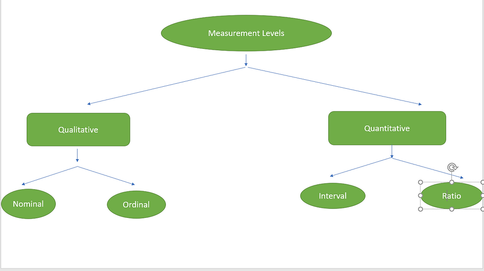
1. Ratios : Ratios has true Zero(0) and Intervals don't.

EX: A has 2 apples vs B has 6 Apples. Which is 3 times as many as B.

Ration of 6/2 is 3.

2. Interval doesn't have zero.

Usually temperature is expressed in celsius or Fahrenheit. They are both interval variables say today is five degrees celsius or 41 degrees Fahrenheit. and yesterday was 10 degrees celsius or 50 degrees fahrenheit terms of celsius, it seems today is twice colder.

Question 1:

1. A variable represents the gender of a person. What type of data does it represent?

Ans : Nominal

2. A variable represents the weight of a person. What type of data does it represent?

Ans : Ordinal

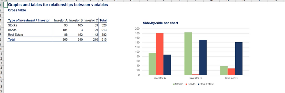
Representation of Categorical Variables

1. Frequency Distribution Table

2. Bar Charts

3. Pie Chart

Relative Frequency:

1. Relative Frequency : Is the percentage of the total frequency for each category.

2. A Pareto diagram is a special type of bar chart, where categories are shown in descending order of frequency.

3. Frequency is the number of occurrences of each item.

4. Cumulative frequency is the sum of the relative frequency.

Step 2: When we have a data set of 20 numbers, I.E the frequency of 1, as each number occurs exactly 1 time. This table would be impractical Hence we group the data.

Intervals largely depends on the amount of data we are working with. In our example, In the above examples we will divide the data into 5 intervals of equal length.

formulae : largest number - smallest number/number of desired intervals.

I.E in our example : Desired intervals interval width = 100-1/5 = 19.8 round off(20)

relative frequency = Frequency/Total Frequency

The most common graph to represent the numerical data is histogram.

Outliers : Outliners are data points that go against the logic of the whole dataset.

* Measures Of Central Tendency

Mean, Median and Mode

Population Mean : μ

Sample :  x̄

How do we find the mean : By adding up all the components and then dividing by the number of components.

Σ : Sum of all values or X

n = Number of observations.

1. It has a huge downside - it is easily affected by outliers.

Lets aid ourselves with an example. These are the prices of pizza at 11 different locations in New York city. and 10 different locations in LA.

The problem in the above example is that we have included an outlier numbers which us doubling the pizza cost in NY. This double the mean.

Median

In order to create the median we need to order the data in ascending order.

The media in the number at position (n+1)/2 in the ordered list.

Mode : Mode is the value that occurs most often.

When each value appears only once. Then there will be no Mode.

Which measure is best?

There is no best, but using only one is definitely the worst.

Weighted Average.

Definition 1: The weighted arithmetic mean is similar to an ordinary arithmetic mean,

except that instead of each of the data points contributing equally to the final average, some data points contribute more than others.

Definition 2 : A weighted mean is a kind of average. Instead of each data point contributing equally to the final mean, some data points contribute more “weight” than others. If all the weights are equal, then the weighted mean equals the arithmetic mean (the regular “average” you're used to).

Formula :

Example : 1

Using the information show below, calculate the final semester grade of John and kelly.

In the above example, John has higher final semester grade than kelly. Because John has score very well in the higher weightage I.E in Test and Final exam compared to Kelly.

Skewness :

The most commonly used tool to measure asymmetry is skewness. This is the formula to calculate.

Skewness indicates whether the data is concentrated on one side.

1. Positive (Right)

2. Zero (No Skew)

3. Negative (Left)

Skewness tell us lot about where the data is situated.

Right Skewness

Zero Skewness

Left Skewness

* Variance : Variance measures the dispersion of a set of data points around their mean.

1. Population variance

• σ2 = population variance

• Σ = sum of…

• Χ = each value

• μ = population mean

• Ν = number of values in the population.

* Sample Variance:

• s2 = sample variance

• Σ = sum of…

• Χ = each value

• x̄ = sample mean

• n = number of values in the sample

Examples :

Variance

Population

1

2

3

4

5

Mean:

=1+2+3+4+5/5 = 3

Population Variance :

Square of (Observation - Mean)

=(1-3)^2+(2-3)^2+(3-3)^2+(4-3)^2+(5-3)^2/5

Result : 2

Sample Variance :

= (1-3)^2+(2-3)^2+(3-3)^2+(4-3)^2+(5-3)^2/(5-1)

Result : 2.50

Note : Reducing the sample n to n – 1 makes the variance artificially large, giving you an unbiased estimate of variability: it is better to overestimate rather than underestimate variability in samples.

Standard Deviation and Co-efficient of variation

Standard deviation : A standard deviation (or σ) is a measure of how dispersed the data is in relation to the mean. Low standard deviation means data are clustered around the mean, and high standard deviation indicates data are more spread out.

Population Standard Deviation Formula

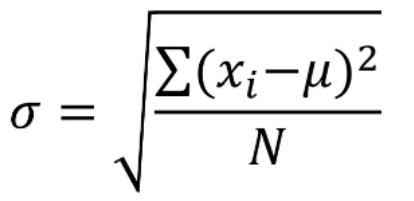
Sample Standard Deviation Formula.

Example : The below examples provides the information of Mean I.E Average, Sample Variance, Sample Standard deviation and co-efficient of variation of the pizza prices of two different countries.

* Standard deviation is the preferred measure of variability, as it is directly interpretable.

Based on the above example, we can come to a conclusion that. We have slightly high variability of prices, evident from the coefficients of variation. In US the value is 0.51, while in India it is 0.60. Note that we only needed the coefficient of variation, because the currencies we used were different.

Distributions with a coefficient of variation to be less than 1 are considered to be low-variance, whereas those with a CV higher than 1 are considered to be high variance.

Co-efficient of variation : The coefficient of variation (CV) is a measure of relative variability. It is the ratio of the standard deviation to the mean (average).

Precise Definition : The coefficient of variation (CV) is the ratio of the standard deviation to the mean. The higher the coefficient of variation, the greater the level of dispersion around the mean. It is generally expressed as a percentage. The lower the value of the coefficient of variation, the more precise the estimate.

• σ – the standard deviation

• μ – the mean

Example : 2 Coefficient of variation

Fuel prices (per gallon) were surveyed every week for 5 weeks in the US and in vietnam. Which country experiences the greatest fuel price fluctuations?

If we looked at those standard deviations, We would think that the fuel prices in India have much higher variation than fuel prices in USA. But actual scenario will be clear, if we look at the coefficient of variation. USA 0.06 and India 0.03, so in this case it seems that fuel prices in USA fluctuate more than fuel prices in India with the above example.

Important : CV is more appropriate when we want to compare between two different data-sets (different units), which has less or more spread. Whereas standard deviation is helpful for us to compare the spread similar types of data sets (same unit).

Example 3:

1. Decide whether you have to use sample or population formula for the standard deviation and the coefficient of variation.

2. Calculate the standard deviation of income in the USA and in Denmark.

3. Calculate the coefficient of variation of income in the USA and in Denmark.

4. Try to interpret the numbers you got.

Ans : The question is asking if this is a sample or a population. In other words, are those all the people in the US or Denmark, receiving salaries? - Obviously not. This is a sample, drawn from the population of all working people respectively in the USA and Denmark.

Coefficient of variation = SD/Mean.

Observation based on the above analysis.

1. Denmark is a much more egalitarian country than the USA.

2. Not only the variance is smaller, but also the standard deviation of salaries.

3. You can get the feeling that almost all people in the country gravitate around the same income.

4. We can further calculate the median income to see if they differ.

5. According to this sample, the average salary in the US is much higher ( $ 189,848 to 504,929.85 kr. = $75,642.41)

6. However, on the average American earns less than the average Danish, which is evident from the median salary.

7. Finally, the coefficients of variation of the salaries in the two countries are very different.

8. In the USA we have much higher variability of income, evident from the coeffcients of variation. In the USA the value is 1.92, while in Denmark it is 0.09.

9. By all means, a coefficient of variation of 1.92 is extremely high, while 0.09 is extremely low.

Notes: Note that we only needed the coefficient of variation, because the currencies we used were different.

Had the salaries been in expressed in dollars for both datasets, a comparison of the standard deviations would be sufficient.

* Covariance:

Covariance is a measure of how much two random variables vary together. It's similar to variance, but where variance tells you how a single variable varies, co variance tells you how two variables vary together.

Calculation procedure.

1. First we have calculated the values for each price and size.

2. Then summed all these values I.E(351992000).

3. The sample size of the below example is 5.

4. Cov. Sample is calculated as follows: summed value divided by sample size - 1 I.E (351992000/(5-1))

Covariance gives a sense of direction.

> 0, the two variables move together

< 0, the two variables move in opposite directions

=0, the two variables are independent.

In covariance values we might results with completely different scale numbers like 5, 0.2999, 33,717,818 etc. How can we interpret these values. That is being explained by correlation coefficient.

* Correlation Coefficient

Correlation adjusts covariance, so that the relationship between the two variables becomes easy and intuitive to interpret.

Formula :

COV(X,Y) / Stdev(X) * Stdev(Y)

Correlation coefficient 1 = Perfect positive correlation.

Correlation coefficient of 0 = Absolutely Independent variables.

Negative Correlation coefficient of -1 = Perfect negative correlation.

Inferential Statistics

Inferential statistics refers to methods that rely on probability theory and distributions, in particular to predict population values based on sample data.

Why do we need inferential statistics?

Consider the case where you are interested in the average number of hours children watch television per day. Now you know that the children in your locality on an average watch television for 1 hour per day. How do you go about finding this for all the children?

There are 2 methods you could use to calculate the results:

1. Collect data about each and every child. 2. Use the data we have to calculate the overall average.

* The first method is extremely difficult and daunting task. The amount of effort and resources required to complete this task would be enormous.

* The second method is much simpler and easier to accomplish. But there is a problem. You cannot equate the average you obtained from a limited data set to the entire population.

* Consider the case where the children in your locality are more interested in sports so the number of hours they spend on television is significantly lesser than that of the overall population. How do we go about finding the population mean?

This is where inferential statistics comes to our rescue.

Inferential Statistics:

Inferential statistics helps us answer the following questions:

* Making inferences about a population from a sample

* Concluding whether a sample is significantly different from the population. Let’s look at the previous example where I pointed out that the sample is different from the population as the children are more interested in sports rather than watching television.

* If adding or removing a feature from a model will help in improving it.

* If one model is significantly different from the other.

* Hypothesis Testing.

This shows us why inferential statistics is important and why it is worth investing time and effort in learning these concepts.

In statistics distribution = probability distribution.

ex: Normal, Binomial and Uniform distribution.

A distribution is a function that shows the possible values for a variable and how often they occur.

ex: Rolling A Die.

1,2,3,4,5,6 occurs once at a time hence the probability value is 1/6 (0.17).

Normal Distribution (Gaussian Distribution) and Z — Statistic:

The normal distribution is also known as the bell curve having the following properties:

1. mean = median = mode.

2. The curve is symmetric with half of the values on the left and half of the values on the right.

3. The area under the curve is 1.

---> Shape of a standard

In a normal distribution:

• 68% of the data falls within one standard deviation of the mean

• 95% of the data falls within two standard deviations of the mean

• 99.7 % of the data falls within three standard deviations of the mean.

Points to be remember:

1. Parameter : A number that describes the data from a population.

2. Statistics : A number that describes the data from a sample.

For calculating the probability of occurrence of an event we need the z — statistic. The

formula for calculating the z — statistic is.

* where x is the value for which we want to calculate the z — value.

* μ and σ are the population mean and standard deviation respectively.

* Basically what we are doing here is standardizing the normal curve by moving the mean to 0 and converting the standard deviation to 1.

* The z — statistic is essentially the distance of the value from the mean calculated in standard deviation terms. So a z — value of 1.67 means that the value is 1.67 standard deviations away from the mean in the positive direction.

* We then find the probability by looking up the corresponding z — value from the z table.

* Deviation score :

Deviation Score = Z * SD

Conclusion:

1. A Z score is the number of standard deviations by which the raw score is above or below the mean.

Questions

1. If a person has an IQ of 125, what percentage of people have higher IQ's.

IQ Scores where M = 100 and SD = 15.

Ans: Z = (x-m)/SD

(125-100)/15 = +1.67.

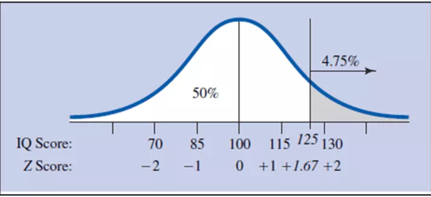
1. 1.67 in the Z column goes with 4.75 in the % in tail column.

2. With a Z score of 1.67, the number of scores above it has to be somewhere between 16% and 2%.

Continued..............................................................................................................................................................