Descriptive Statistics - Linear Regression (Least Squared Method)

Definition :

Linear regression analysis is used to predict the value of a variable based on the value of another variable. The variable you want to predict is called the dependent variable I.E (Y). The variable you are using to predict the other variable's value is called the independent variable (X).

In this article, I will explain about linear regression using the least squared method with an example set and this approach will help us to write the linear equation that best fits the data in the table show below.

Least Square Method : The least-squares method is a statistical procedure to find the best fit for a set of data points by minimizing the sum of the offsets or residuals of points from the plotted curve. Least squares regression is used to predict the behavior of dependent variables.

1. The following visual illustrates the linear regression chart for the following attributes.

X : Number of Orders (Independent Variable) and Man Power Y : (Dependent Variable).

In the following example we're trying to predict the required man power based on the number of orders recorded. Using linear regression least squared method.

* To predict the required man power first we need to calculate the equation. That can be achievable using data analysis inbuilt function in excel. But lets calculate it using formula method for better understanding.

Basics :

* B0 : Represents the intercept

* B1 : Represents the slope of the regression line.

* Linear Equation formula :

y = mx + b (Algebra)

(y = b0 + b1*x) (Statistics)

slope = m = b1 ------ y Intercept = b = bo

Step 1

m = n Σxy - Σx Σy / n Σ x² - (Σ x)²

I'm applying the formula values based on the details which I have specified in the excel

Numerator

n = number of values I,E : 19

Σ xy = Multiplying X and Y values

Σx : sum of x values

Σy : sum of y values

Denominator

n : Number of values

Σ x² : sum of X squared values

(Σ x)² : Squaring the sum of x values.

Formula simplification

=19*(16289901) - (128139)*(2182) / 19 (1003465421) - (128139)^2

Result : 0.0113

Step 2

b = Σ Y - m Σ x / N

Σ Y : Sum of y values, Σ x : sum of x values, N = number of values

=(2182) - (0.0113)*(128139) / 19

Result : 38.61

* Linear equation will be

y = m x + b

y = 0.0113x + 38.61.

Equation Sample & Explanation :

(Y = mx+b) = (Y = b0+b1x) --(slope m = b1), (y intercept b = b0)

To find the (slope m = b1)

Formula:

To find the (y intercept b = b0)

Final overview

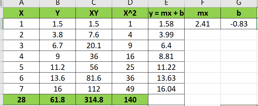
y = 2.41 X - 0.83

Based on this linear equation, I have calculated the following details in the excel.

1. Forecast- Linear Regression (Predicted Value) : Applied the same equation and calculated the forecasted result of this equation. (=0.0113x + 38.61 & X)

2. R- Square : SSR - Sum of squares due to regression / SST - Sum of Squares Total.

3. SSR Sum of squares due to regression : Forecast value (Predicted value) - Y Mean(Man Power mean)

4. SST - Sum of squares total : Y Variable (Man Power value) - Y Mean (Man power mean) . * What is SST? The sum of squares total, denoted SST, is the squared differences between the observed dependent variable and its mean. You can think of this as the dispersion of the observed variables around the MEAN.

It is a measure of the total variability of the dataset. Note: There is another notation for the SST. It is TSS or total sum of squares.

* What is the SSR?

The second term is the sum of squares due to regression, or SSR. It is the sum of the differences between the predicted value and the mean of the dependent variable. Think of it as a measure that describes how well our line fits the data.

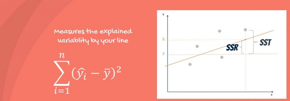
If this value of SSR is equal to the sum of squares total, it means our regression model captures all the observed variability and is perfect. Once again, we have to mention that another common notation is ESS or explained sum of squares.

3. What is the SSE?

The last term is the sum of squares error, or SSE. The error is the difference between the observed value and the predicted value.

We usually want to minimize the error. The smaller the error, the better the estimation power of the regression. Finally, I should add that it is also known as RSS or residual sum of squares.

R-squared is a statistical measure of how close the data are to the fitted regression line.

If our example data set r-square is 0.98 which is strongly correlated.

Standard Error Estimate : sum of all the (Predicted value - Y mean)/number of variables - 2 I.E 3.76. (Approximately how much error you make when you use the predicted value for Y).

Multiple Linear Regression :

It explains the relationship between two or more independent variables and a response variable by fitting a straight line.

In the Article we are trying to predict the sales based on the following attributes. TV Marketing, Radio Marketing, New_Paper Marketing.

A multiple regression model has the form: Y = B0 + B1 * Tv_marketing +B2 * Radio marketing + B3 * newspaper marketing. Sales are in crores and the budget is in lakhs

Multiple Linear Regression Equation will be : = Y = 2.859 + TV_Marketing value * (0.0055) + Radio_Marketing value * (0.1688) + Newspaper marketing value * (-0.0152)

Newspaper marketing is having negative coefficient. (TV_Marketing and Radio_Marketing) are positive coefficient.

Now we understood that not all variables are useful to build a model. Some independent variables are insignificant and add nothing to your understanding of the outcome/ response/ dependent variable. In the case of the sales prediction problem, the variable Newspaper marketing was insignificant. Thus, the final model had only two significant variables, i.e. Radio marketing and TV marketing.

P-value :

p > 0.05 : Fail to reject the hypothesis and variable is insignificant.

p < 0.05 : Reject hypothesis, Variable is significant.

Question : In a model containing multiple independent variables, which variables would be insignificant and need to be removed from your model?

Answer : p>0.05 means that you fail to reject the null hypothesis, i.e. null hypothesis is true that the variable is insignificant. So you will remove variables with higher p-value.

------------------------------------------------------------------------------------------------------------------------------------

Statistics

* Mean, Median and Mode:

Mean :

Σ : Sum of all values or X

n = Number of observations.

Definition 1: The weighted arithmetic mean is similar to an ordinary arithmetic mean,

except that instead of each of the data points contributing equally to the final average, some data points contribute more than others.

Definition 2 : A weighted mean is a kind of average. Instead of each data point contributing equally to the final mean, some data points contribute more “weight” than others. If all the weights are equal, then the weighted mean equals the arithmetic mean (the regular “average” you're used to).

Formula :

Example : 1

Using the information show below, calculate the final semester grade of John and kelly.

In the above example, John has higher final semester grade than kelly. Because John has score very well in the higher weightage I.E in Test and Final exam compared to Kelly.

* Variance : Variance measures the dispersion of a set of data points around their mean.

1. Population variance

• σ2 = population variance

• Σ = sum of…

• Χ = each value

• μ = population mean

• Ν = number of values in the population

• 
  

* Sample Variance:

• s2 = sample variance

• Σ = sum of…

• Χ = each value

• x̄ = sample mean

• n = number of values in the sample

Examples :

Variance

Population

1

2

3

4

5

Mean:

=1+2+3+4+5/5 = 3

Population Variance :

Square of (Observation - Mean)

=(1-3)^2+(2-3)^2+(3-3)^2+(4-3)^2+(5-3)^2/5

Result : 2

Sample Variance :

= (1-3)^2+(2-3)^2+(3-3)^2+(4-3)^2+(5-3)^2/(5-1)

Result : 2.50

Note : Reducing the sample n to n – 1 makes the variance artificially large, giving you an unbiased estimate of variability: it is better to overestimate rather than underestimate variability in samples.

* Standard Deviation and Co-efficient of variation:

Standard deviation : A standard deviation (or σ) is a measure of how dispersed the data is in relation to the mean. Low standard deviation means data are clustered around the mean, and high standard deviation indicates data are more spread out.

Population Standard Deviation Formula

Sample Standard Deviation Formula.

Example : The below examples provides the information of Mean I.E Average, Sample Variance, Sample Standard deviation and co-efficient of variation of the pizza prices of two different countries.

Based on the above example, we can come to a conclusion that. We have slightly high variability of prices, evident from the coefficients of variation. In US the value is 0.51, while in India it is 0.60. Note that we only needed the coefficient of variation, because the currencies we used were different.

Distributions with a coefficient of variation to be less than 1 are considered to be low-variance, whereas those with a CV higher than 1 are considered to be high variance.

Co-efficient of variation : The coefficient of variation (CV) is a measure of relative variability. It is the ratio of the standard deviation to the mean (average).

Precise Definition : The coefficient of variation (CV) is the ratio of the standard deviation to the mean. The higher the coefficient of variation, the greater the level of dispersion around the mean. It is generally expressed as a percentage. The lower the value of the coefficient of variation, the more precise the estimate.

• σ – the standard deviation

• μ – the mean

Example : 2 Coefficient of variation

Fuel prices (per gallon) were surveyed every week for 5 weeks in the US and in vietnam. Which country experiences the greatest fuel price fluctuations?

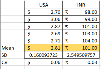
If we looked at those standard deviations, We would think that the fuel prices in India have much higher variation than fuel prices in USA. But actual scenario will be clear, if we look at the coefficient of variation. USA 0.06 and India 0.03, so in this case it seems that fuel prices in USA fluctuate more than fuel prices in India with the above example.

Important : CV is more appropriate when we want to compare between two different data-sets (different units), which has less or more spread. Whereas standard deviation is helpful for us to compare the spread similar types of data sets (same unit).

* Covariance:

Covariance is a measure of how much two random variables vary together. It's similar to variance, but where variance tells you how a single variable varies, co variance tells you how two variables vary together.

Covariance gives a sense of direction.

> 0, the two variables move together

< 0, the two variables move in opposite directions

=0, the two variables are independent.

* Correlation Coefficient

Correlation adjusts covariance, so that the relationship between the two variables becomes easy and intuitive to interpret.

Formula :

COV(X,Y) / Stdev(X) * Stdev(Y)

Correlation coefficient 1 = Perfect positive correlation.

Correlation coefficient of 0 = Absolutely Independent variables.

Negative Correlation coefficient of -1 = Perfect negative correlation.

* Logistic Regression:

In Linear regression. Our prediction value is continuous like home prices, weather and stock price. Where as in logistic regression the prediction value is categorical.

ex: 1. Will customer buy insurance Yes/No,

2. Email is spam or not.

3. Which party a person is going to vote for?

A. Democratic B. Republican C. Independent

4. Is an individual transaction fraudulent or not?

5. What Determines admittance into a school?

6. Which customers are more likely to buy a new product?

Predicted value is categorical.

Logistic Regression is one of the techniques used for classification.

Classification Types :

1. Binary Clarification :

Ex: Will customer buy insurance Yes/No.

2. Multiclass Classification :

Ex: Which party a person is going to vote for?

A. Democratic B. Republican C. Independent

In Logistic Regression : The data is being depicted based on the sigmoid or logit function.

Sigmoid Function :

e = Euler's number ~ 2.71828

Here we are dividing 1 by A number which is slightly greater than 1. In this situation the outcome will be less than 1.

Sigmoid or logit function converts input into range 0 to 1. The equation that we get that looks like S shape function.

Linear regression vs Logistic Regression.

1. Linear Regression predicted values is continuous where as the logistic regression predicted values is categorical (Whether customer buys Insurance Yes/No).

Pre-requisites

Exponents : An exponent refers to the number of times a number is multiplied by itself.

ex:

* 3^2 (3 raised to 2) i.e 3*3 = 9.

* 3^4 (3 raised to 4) i.e 3*3*3 = 27.

here 3 is the base and 4 is exponent

Negative exponents

1. 3^-4

2. 3^-4 * 3^4/3^4 (product law)

-4 and +4 get cancelled and 3^0/3^4.

Any non zero number raised to 0 equals 1.

Final Answer: 1/3^4.

In simple terms just change the negative sign to positive sign.

ex: (21/37)^-7 = 1/(21/37)^7

Logarithms : Logarithms are the inverse of exponents. A logarithm (or log) is the mathematical expression used to answer the question: How many times must one “base” number be multiplied by itself to get some other particular number?

For instance, how many times must a base of 10 be multiplied by itself to get 1,0000?

Ans : 10^4.

ex:

1. 3^4 = 81

log3(81) = 4

(logarithm of 81 to the base 3) = 4

ex: log5(125) = X

2. 5^X = 125

5^5 = 12 hence x= 5

3. log4(1) = y

4^y = 1

(Any non-zero number)^0 = 1

4^0 = 1

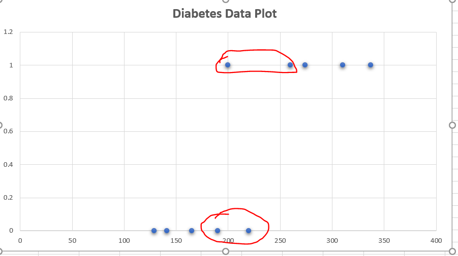
In this article we're trying to predict the whether a person is diabetic or not based on the blood sugar level.

Here diabetes is a categorical variable and we code this as follows.

(No as 0). (Yes as 1).

Here on X axis we have plotted the Blood sugar level and on Y axis summary Diabetes (Yes = 1) or (No = 0).

Based on the decision boundary line we can't predict the diabetes. Because we may miss classify few patients as show in the diagram.

I.E suppose if we consider blood sugar > 210 as diabetic and patients sugar level < 210 don't have diabetics. Here we may misclassify 2 patients.

So conclusion here is using a simple boundary decision method would not work in this case.

The ways of overcoming from these problem is different probabilities as follows.

1. The patients whose blood sugar level is extremely very low. We want the probability of a person being diabetic with this sugar level to be very very low.

2. The patients blood sugar level is extremely very high and high probability that person is diabetic.

3. For intermediate points where the sugar level in the range of no high or low there we would like to have some probability of 0.5 or 0.6.

----------------------------------------------------------------------------------------------------------------------------------------

Sigmoid Curve

Y(Probability of Diabetes) =

1/1 + e^-(b0+b1x)

Sigmoid curve has all the properties i.e - extremely low values in the start, extremely high values in the end, and intermediate values in the middle. It’s a good choice for modelling the value of the probability of diabetes.

However, you may be wondering why can’t we just fit a straight line here? This would also have the same properties - low values in the start, high ones towards the end, and intermediate ones in the middle.

The main problem with a straight line is that it is not steep enough. In the sigmoid curve, as you can see, you have low values for a lot of points, then the values rise all of a sudden, after which you have a lot of high values. In a straight line though, the values rise from low to high very uniformly, and hence, the “boundary” region, the one where the probabilities transition from high to low is not present.

Now let us learn how to find the best fit sigmoid curve. (β 0 and β 1 which fits the data best).

Sigmoid Curve

We have provided a alphanumeric character for each data point as (P1, P2, P3, P4,P5,P6,P7,P8,P9,P10).

P4 : 4th data point, we want p4 to be as low as possible because he is not a diabetic and similarly for p3,p2 and p1 as well as p6.

For P5,P7,P8,P9,P10 the probability of being diabetic is large hence we want the curve as large as possible

The best fitting combination of β 0 and β 1 will be the one which maximises the product:

(1−P1)(1−P2)(1−P3)(1−P4)(1−P6)(P5)(P7)(P8)(P9)(P10).

It is the product of:

[(1−Pi)(1−Pi)------ for all non-diabetics --------] * [(Pi)(Pi) -------- for all diabetics -------]

.

The ten points in our example, the labels are a little different, somewhat like this.

Finding the best fit sigmoid curve.

If we had to find β 0 and β 1 for the best fitting sigmoid curve, you would have to try a lot of combinations, unless you arrive at the one which maximises the likelihood. This is similar to linear regression, where you vary β 0 and β 1 until you find the combination that minimises the cost function. Hence, this is called a Generalised Linear regression Model (GLM), or a logistic regression model.

So, just by looking at the curve here, you can get a general idea of the curve’s fit. Just look at the yellow bars for each of the 10 points. A curve that has a lot of big yellow bars is a good curve.

Clearly, this curve is a better fit. It has many big yellow bars, and even the small ones are reasonably large. Just by looking at this curve, you can tell that it will have a high likelihood value.

Will be Continued................................... with more granular examples in next sessions.